Circuit simulation

Frequency-domain simulation

Circuit simulation in the frequency domain can be done in two ways with IPKISS:

1. Through Python scripting. This allows for a unified workflow where simulation and layout are defined together within IPKISS.

2. Using the Luceda Layout Visualizer with a SPICE netlist. You can launch the visualizer from the Luceda Control Center or from code.

Our simulation is layout-driven, which means that the simulation model is directly derived from the spice file associated to the physical layout. This ensures a close match between the simulated performance and the behavior of the fabricated device.

Python script based frequency-domain simulation

Let us start with an example of a simulation configured via a Python script. If every component in a circuit has a model attached to it, running a frequency-domain simulation is quite simple. Let’s start with the two-level splitter tree from the previous chapter as an example. As always, we first import the PDK, IPKISS, and any other dependencies we need:

from si_fab import all as pdk  # noqa: F401
from ipkiss3 import all as i3
import matplotlib.pyplot as plt
import numpy as np
from circuits_to_simulate import SplitterTree  # importing the circuit we want to simulate

Because every MMI and waveguide in SiFab has a predefined model already, we just need to instantiate the CircuitModelView of the circuit and call get_smatrix:

circuit = SplitterTree()  # instantiate our basic SplitterTree circuit

circuit_model = circuit.CircuitModel()  # instantiate our SplitterTree circuit model
wavelengths = np.linspace(1.5, 1.6, 501)  # create an array of wavelengths for simulation in units of micrometers

S_total = circuit_model.get_smatrix(wavelengths=wavelengths)

The result is an S-matrix describing the transmission between any two ports, and can be visualized using Matplotlib or a dedicated visualizer. The usage of Matplotlib is shown below. We see that the power is split evenly among the outputs and there are some small reflections at the input.

plt.plot(wavelengths, i3.signal_power_dB(S_total["out1", "in"]), linewidth=2, label="out1")
plt.plot(wavelengths, i3.signal_power_dB(S_total["out2", "in"]), linewidth=2, label="out2")
plt.plot(wavelengths, i3.signal_power_dB(S_total["out3", "in"]), linewidth=2, label="out3")
plt.plot(wavelengths, i3.signal_power_dB(S_total["out4", "in"]), linewidth=2, label="out4")
plt.xlabel(r"Wavelength [$\mu$m]", fontsize=16)  # add a label to the x-axis
plt.ylabel("Transmission [dB]", fontsize=16)
plt.ylim([-10, 0])
plt.legend(fontsize=14)  # create a legend from the plt.plot labels
plt.show()  # show the graph

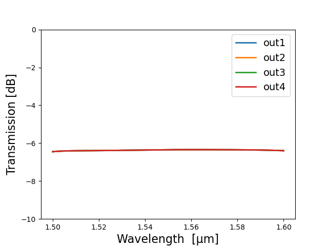
Frequency-domain simulation of a two-level splitter tree design: transmission

An easier way to plot the results of an S-matrix frequency sweep is to use the dedicated visualize method. This will open the interactive Luceda S-matrix Visualizer, where users can explore the S-parameters from/to each port, toggle linear and logarithmic scales, and customize the styling of the plots.

    S_total.visualize(
        term_pairs=[("in", "in"), ("in", "out1"), ("in", "out2"), ("in", "out3"), ("in", "out4")],
        scale="dB",
        ylabel="Transmission [dB]",
    )

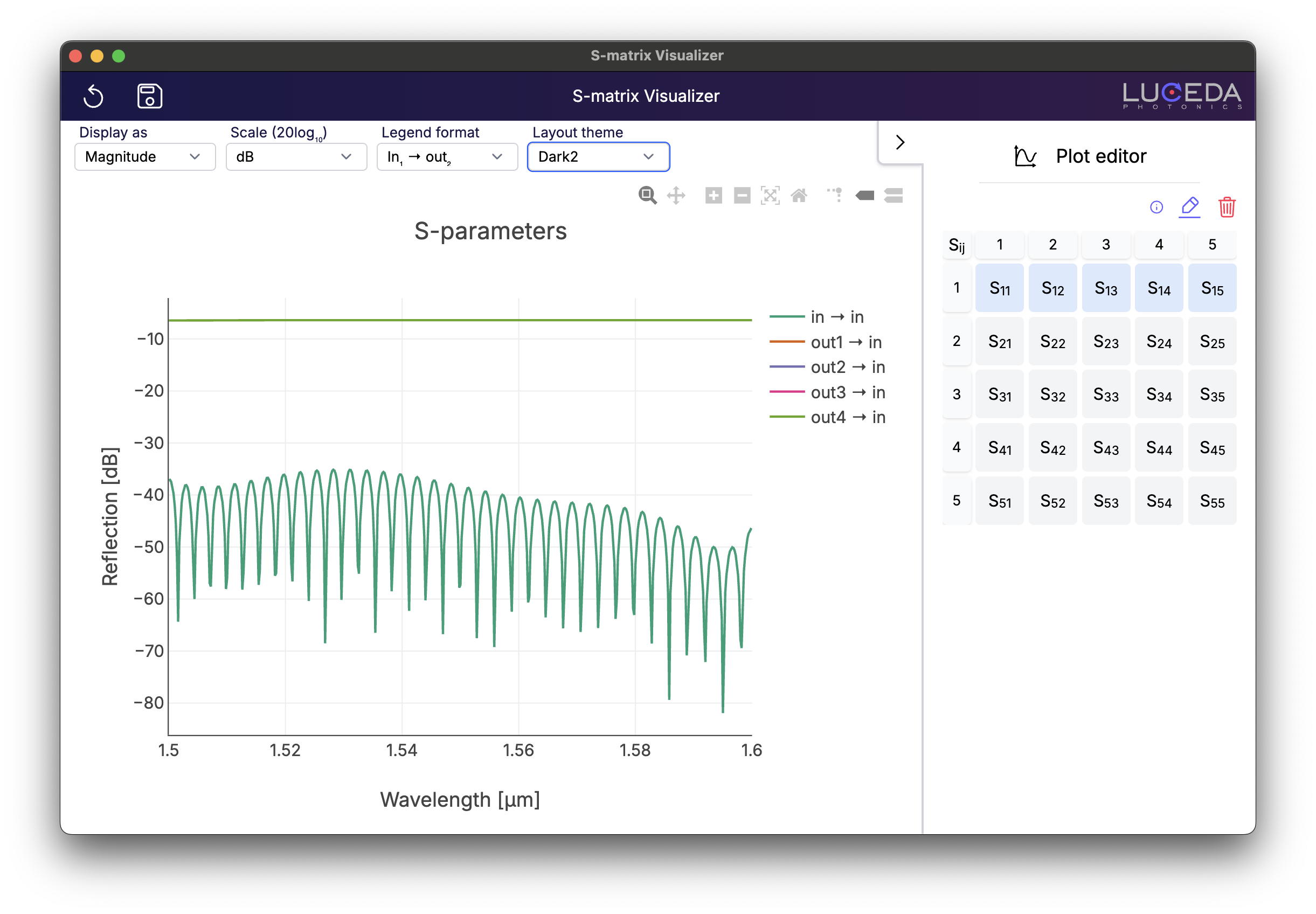
The Luceda S-matrix Visualizer displaying the results of the splitter tree (reflection + transmissions).

Running these simulations in a code environment provides interesting possibilities. We can, for example, use for-loops to sweep a parameter’s value and find out how it impacts the circuit’s performance. This can be demonstrated with a Mach-Zehnder Interferometer (MZI):

mzi = MZI(path_difference=100)
mzi_layout = mzi.Layout()
mzi_layout.visualize(annotate=True)

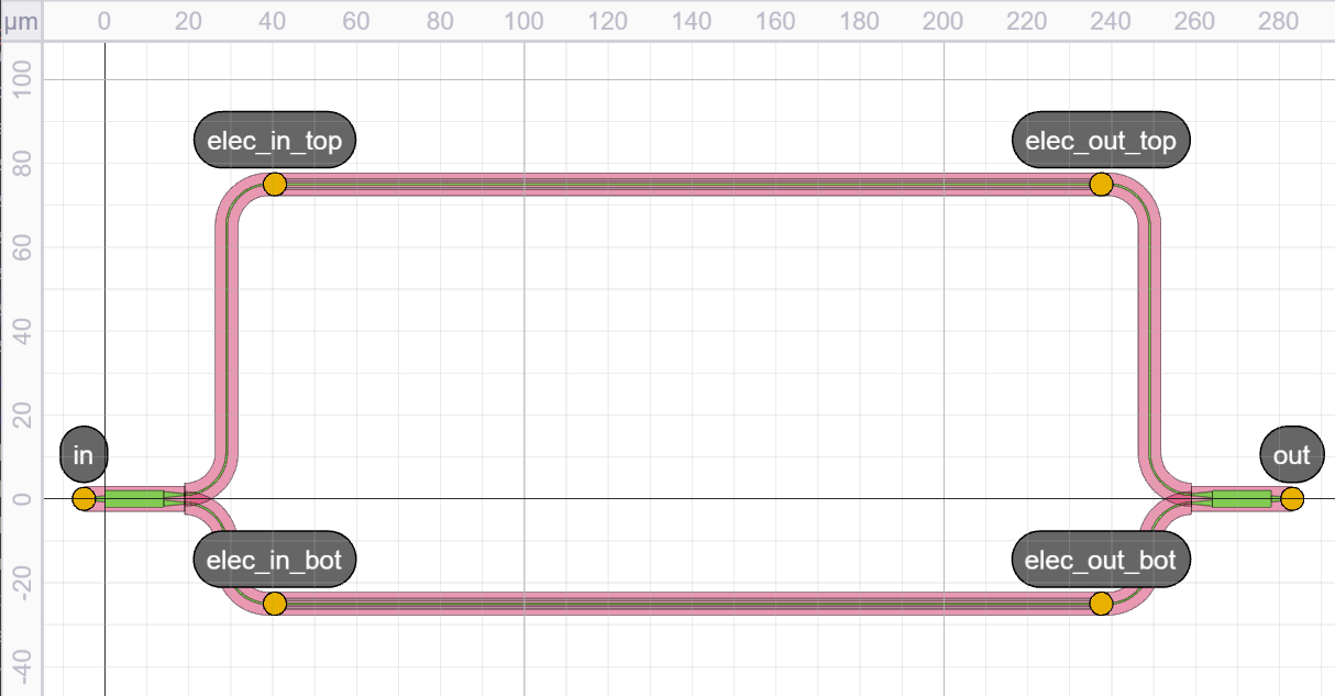
Mach-Zehnder Interferometer with heated top and bottom arm

We will sweep over a range of path length differences between the two arms of the MZI, resulting in different interference patterns at the output:

path_differences = np.linspace(50, 150, 3)  # range from 50 to 150 um, in steps of 50 um

for path_difference in path_differences:  # iterate over "path_differences"
    mzi_model = MZI(path_difference=path_difference).CircuitModel()  # call the CircuitModel() method on each new MZI
    mzi_model.get_smatrix(wavelength_range).visualize(  # calculate and visualize the s_matrix
        term_pairs=[("in", "out")],
        scale="dB",  # convert to dB
        ylabel="Transmission [dB]",
        title=f"path_difference = {path_difference}",  # use f-strings to format the title
    )

Similar to the first example, the result for each value of the path length difference can be plotted. As the path difference increases, the free spectral range decreases proportionally as expected.

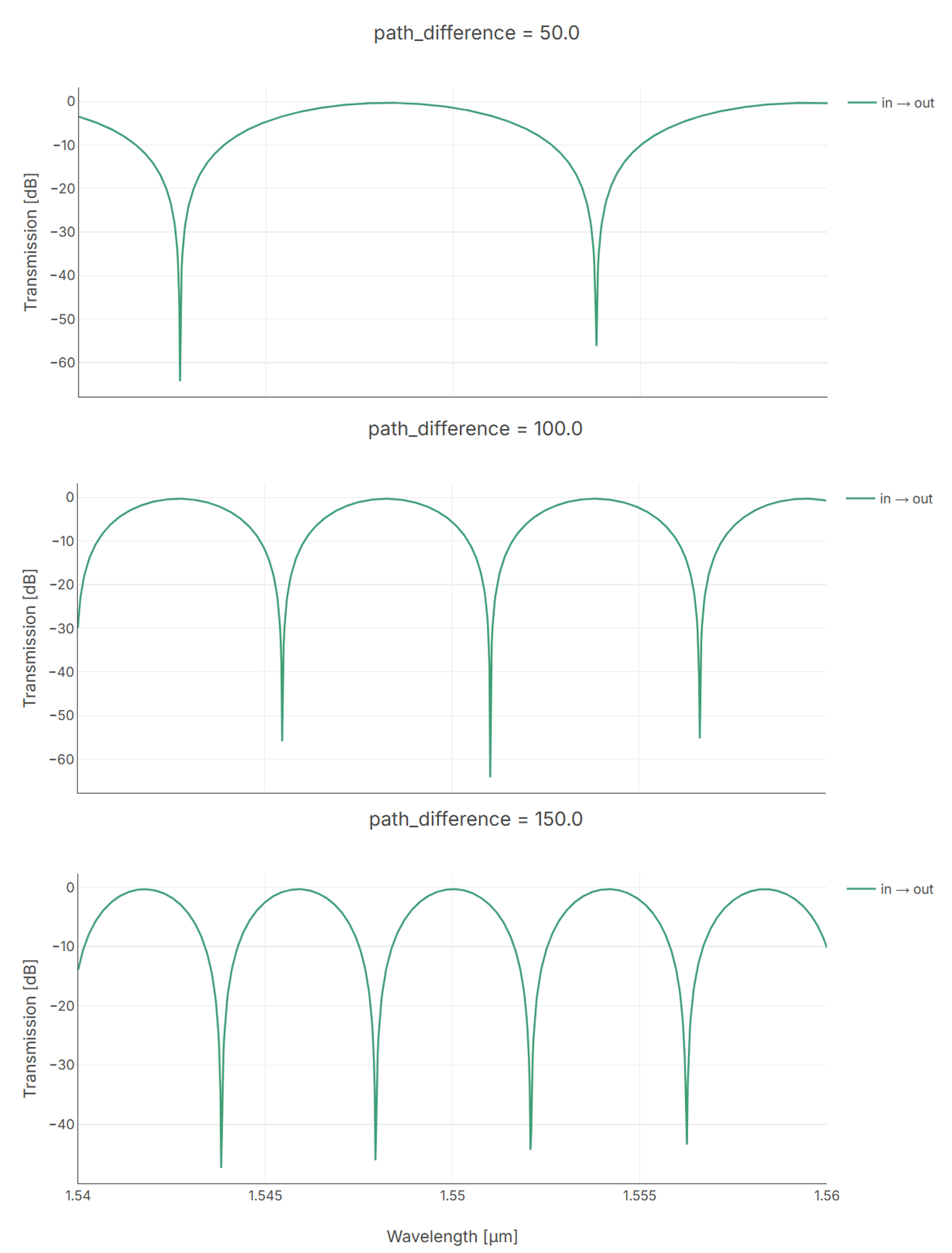
MZI transmission as a function of wavelength for different path length differences between the top and bottom arm

Spice-based frequency-domain simulation

This section explains how to perform circuit simulations using SPICE files. This allows you to import a SPICE file (generated by IPKISS) to run simulations with Caphe on a layout designed in IPKISS. Alternatively, you can import both a GDS file and a SPICE file to run the simulation directly in the Luceda Layout Visualizer (which you can start from the Luceda Control Center).

The SPICE-based approach offers several advantages. It provides interoperability with standard electronic design automation (EDA) tools and makes the simulation configuration self-contained. As long as an appropriate SPICE file is created, you can run simulations independently of the original IPKISS Python design script, which improves reproducibility and collaboration.

Let’s start by creating a SPICE file for our examples and demonstrate the workflow using the Luceda Layout Visualizer. Using the MZI from the previous section, you can create a SPICE file from a circuit with the following code:

mzi = MZI()
mzi_layout = mzi.Layout()
mzi_layout.visualize()

wavelength_range = np.linspace(1.54, 1.56, 1001)

mzi_cm = mzi.CircuitModel()
mzi_cm.get_smatrix(wavelengths=wavelength_range, spice_path="my_mzi.spice")
mzi_cm.to_spice(filename="my_mzi_2.spice")

mzi_layout.write_gdsii("my_mzi.gds")

The code shows two ways of generating a SPICE file. The first method, i3.CircuitModelView.get_smatrix, includes the analysis parameters (like the wavelength range) in the SPICE file itself. The second method, to_spice, only exports the circuit netlist. We will use the first method. If we used the second, we would need to specify the simulation parameters, such as the wavelength range, in the Luceda Layout Visualizer.

Once we have a SPICE file containing the circuit netlist and component models, we are ready to proceed.

Running the script 4_circuit_simulation\1_tutorials\2_mzi_frequency_LDS.py will launch the Luceda Layout Visualizer.

Once the Luceda Layout Visualizer is launched with our MZI layout, you will see a simulation icon in the top bar and also below the Layers tab on the right (highlighted in the figure below).

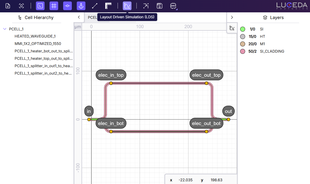
Luceda Layout Visualizer with MZI layout.

Clicking the simulation icon opens the Layout-Driven Simulation panel. The simulation output console will appear at the bottom, showing simulation logs, and the tool will automatically connect to the simulation server.

The panel on the right-hand side contains a “Spice File” section. Here, you can select the path to your SPICE file. We will use the file generated from the code in the previous step.

When a file is added, the tab expands to show more options.

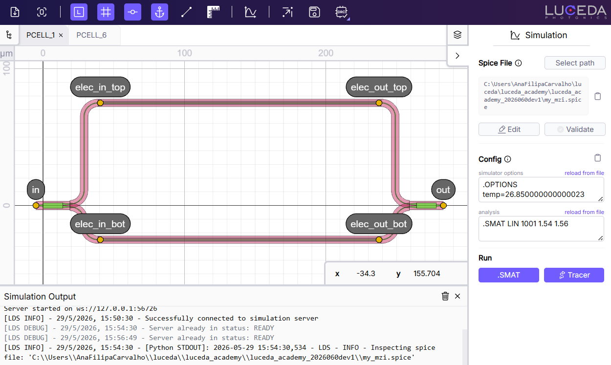
Simulation tab with a selected spice file.

In the “Spice File” section, you can click the “Edit” button to open and edit your SPICE file directly. You can also click “Validate” to perform a check on the SPICE file. If you modify and save the file, the changes will be made available in the Luceda Layout Visualizer. For example, if you click on “reload from file”, the changes to the analysis and options sections will be updated. We recommend validating the file again after making changes and to check the console logs in case the SPICE file is no longer valid.

The last section allows you to run the simulation and visualize the results.

Pressing the SMAT button opens a Visualizer with the S-matrix results, similar to the one generated from Python scripts. In our case, with the default path length difference set to \(100.0\), the results should match the previous plot:

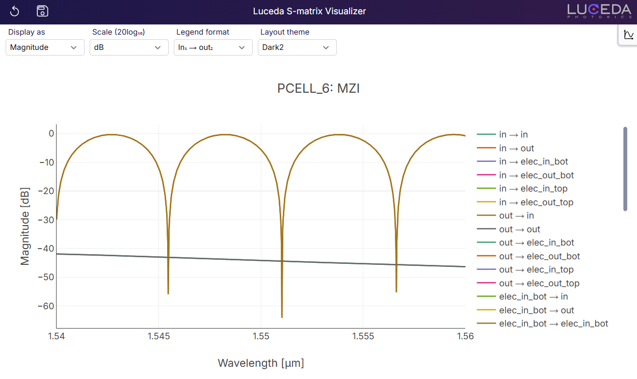
Plot of S-matrix results directly from the Luceda Layout Visualizer.

By using the Plot Editor to show only the transmission from the “in” port to the “out” port, we can reproduce the exact same plot as before.

Pressing “Tracer” will display a Tracer analysis on your layout.

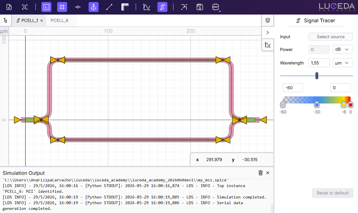
Running Signal Tracer from a SPICE file directly on the layout.

IPKISS takes the layout hierarchy and ports, connects them to the SPICE description, and guarantees that they match.

The Signal Tracer requires additional information that is not present in a GDS. To use it, your layout should be directly exported from IPKISS code.

Note that Signal Tracer is computationally intensive. It is advisable to reduce the number of simulated wavelengths with Signal Tracer.

You can find another example of Tracer in Beneš switch network with Circuit Analyzer.

The “Configuration” section is optional when we give a SPICE file with the analysis section. Here, you can adjust simulator options and wavelength settings, provide the values if they are not specified, or override the values defined in your SPICE file. By default, the simulation uses the settings from the SPICE file. You can revert any changes back to the original file’s values by clicking “reload from file”.

Updating the values here and running the simulation will open a new S-Matrix Visualizer with the new results:

Running simulation from a SPICE file and updating the wavelength range

For another example of a SPICE-based simulation, see the A SPICE-Based Simulation Workflow in IPKISS in our sample gallery. This example also uses the MZI and demonstrates how to use a SPICE file for efficient voltage sweeps.

Time-domain simulation

To conclude, we’ll have a short look at time-domain simulations. These are slightly more complicated than frequency-domain simulations, and fully describing them is out of the scope of a ‘getting started’ course. If you want more information, please visit Creating a First Circuit Simulation.

Both arms of the MZI in the previous example can be thermally tuned by applying a voltage to their electrical ports. If a constant optical signal is sent through the input while the voltage across one of the arms is steadily increased, we expect that the power level at the output will change over time. To test this, let’s start by creating optical and electrical sources:

def ramp_function(t_rise, amplitude):
    """Returns a simple linear voltage ramping function to apply to our circuit. "t" is the current time in the
    simulation, "t_rise" is the time it takes for the voltage to ramp to its maximum, and "amplitude" is the final
    value of the applied voltage.
    """

    def f_step(t):
        if t <= t_rise:
            return amplitude * (t / t_rise)
        else:
            return amplitude

    return f_step

dt = 1e-7  # setting up the time step variable for our simulation
voltage_function = ramp_function(t_rise=70 * dt, amplitude=3.5)  # create our driving voltage function

optical_source = i3.FunctionExcitation(port_domain=i3.OpticalDomain, excitation_function=lambda x: 1)
voltage_drive = i3.FunctionExcitation(port_domain=i3.ElectricalDomain, excitation_function=voltage_function)

Next, similarly to what you would do in a real lab setting, we will create a virtual ‘testbench’ circuit that connects the MZI to the sources and a probe to register the transmission at the output. To make these logical connections we can use i3.ConnectComponents:

circuit = i3.ConnectComponents(
    child_cells={
        "mzm": MZI(path_difference=5.5),  # the circuit we want to simulate
        "src_opt": optical_source,  # the optical source to be used
        "v_drive": voltage_drive,  # the drive voltage excitation
        "opt_out_probe": i3.Probe(port_domain=i3.OpticalDomain),  # our optical monitor
    },
    links=[
        ("v_drive:out", "mzm:elec_in_bot"),  # connect the dc_voltage to one of the electric heaters in the circuit
        ("src_opt:out", "mzm:in"),  # connect the optical source to the MZI optical input
        ("mzm:out", "opt_out_probe:in"),  # connect the optical probe to the MZI optical output
    ],
)

As you can see, the voltage is applied to the bottom arm. The source and probe are connected to the input and output of the MZI respectively.

Finally, we instantiate the CircuitModelView and call get_time_response, passing in our parameters for the start and end times, time step and central wavelength:

result = circuit.CircuitModel().get_time_response(t0=0.0, t1=1e-5, dt=dt, center_wavelength=1.55)

Plotting the result can be done in the following way:

plt.title("MZI thermal tuning in the time domain", size=20)
plt.xlabel("Simulation time steps")
plt.ylabel("Optical output power [dB]")
plt.plot(i3.signal_power_dB(result["opt_out_probe"][1:]))
plt.show()

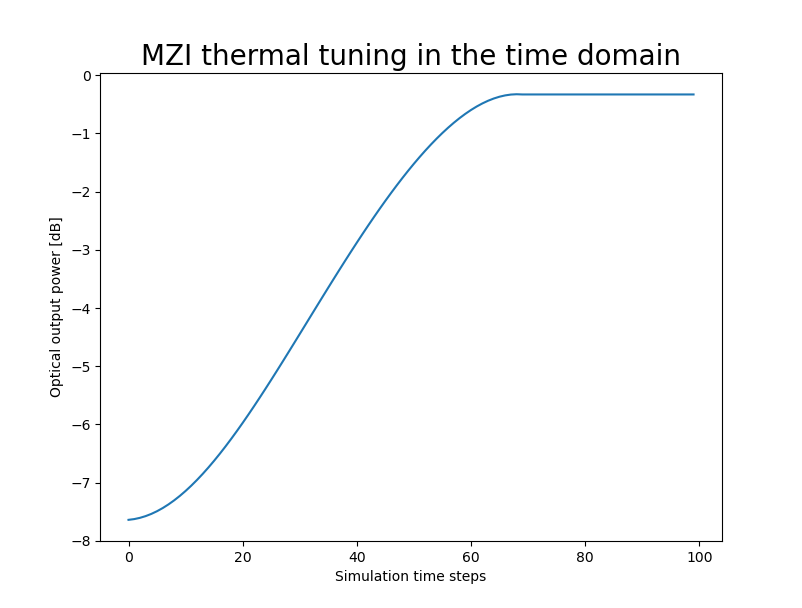
Time-domain simulation of a thermally tuned MZI

As expected, we see the initial transmission is poor due to the imbalance in the path differences. As we apply our ramping voltage, the refractive index in the bottom arm changes, reducing the phase difference and resulting in a higher overall transmission.

More information

• We have purposely left out what the models of our components look like and how to implement them. This is covered in a later section of the “getting started” course: Component models.

• Find out what Caphe has to offer and what its advantages are: Caphe introduction.

Exercise

In getting_started/4_circuit_simulation/2_exercises/exercises.py you will find an incomplete Python script. The purpose of the script is to run a frequency-domain simulation of a circuit with and without grating couplers. To practice what we’ve learned in this chapter, try to fill in the missing code. There is also a solution file in case you get stuck.